|
DEPARTMENT OF ELECTRICAL MACHINES, MARKETING & MANAGEMENT |
|
DEPARTMENT OF ELECTRICAL MACHINES, MARKETING & MANAGEMENT |
Modular hybrid linear and surface stepper motors
The research team:
![]()
The advantages of linear motors
The "classical" hybrid linear stepper
motor
The modular linear motor
![]() Design
Design
![]() The
sample motor
The
sample motor
![]() Magnetic
field analysis
Magnetic
field analysis
![]() Control
Control
![]() Simulation
Simulation
The modular surface motor
![]() Control
Control
![]() Simulation
Simulation
Main
papers published in this field
The main advantage of any linear motor is that it totally eliminates the need, cost and limitations of mechanical rotation-to-translation mechanisms such as racks and pinions or belts and pulley, sources of elasticity and backlash. This way the complexity of the mechanical system is drastically reduced [1].
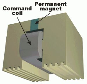
The hybrid liner motor (shown in Fig. 1) is in fact a variable reluctance, permanent magnet excited synchronous motor, having a movable armature (the mover or forcer) suspended over a fixed stator (the platen). The platen is an equidistant toothed bar of any length fabricated from high permeability cold-rolled steel. The mover consists of two electromagnets having command coils and a strong rare earth permanent magnet between them, which serves as a bias source. Each electromagnet has two poles, and all poles, toothed to concentrate the magnetic flux, have the same number of teeth. The toothed structures in both armatures have the same fine teeth pitch. The four poles are spaced in quadrature, so that only one pole at a time can be aligned with the platen teeth.
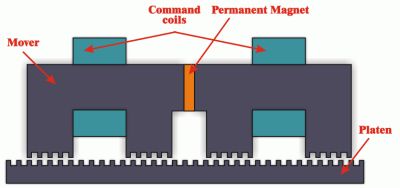
Fig. 1 .
It is operating under the combined principles of variable reluctance and of permanent magnet motors. When current is established in a command coil, the resulting magnetic flux tends to reinforce the flux of the permanent in one pole of that electromagnet and to cancel it in the other. By selectively applying current pulses to the two command coils, it is possible to concentrate flux in any of the poles. The pole receiving the highest flux concentration will attempt to align its teeth with the platen teeth by generating a tangential force, in a manner as to minimise the air-gap magnetic energy. Four steps result in motion of one tooth interval.
The above-presented motor type has some disadvantages. As the electromagnets are not definitely independent, the magnetic flux produced by the command coils flows through the permanent magnet, existing the peril of its demagnetisation. In any position one of the poles is generating a significant breaking force, diminishing the total tangential force produced by the motor and reducing its efficiency. Beside these the magnetic flux passing between the mover and the platen gives rise to a very strong normal force of attraction between the two armatures. This attractive force, produced of all the poles, is over 10 times the peak holding force of the motor, requiring sophisticated bearing systems to maintain the precise air-gap between the mover and platen. The greatest attractive force is generated of the same pole that produced the breaking tangential force (the pole those teeth were aligned with the platen teeth before starting the current step). These disadvantages could be eliminated by reducing significantly the magnetic flux passing through the passive poles (the two poles of that electromagnet of which command coil is not energised) [1].
A possible solution to this problem it could be the innovative modular double salient permanent magnet linear motor [3].
Using modules like that shown in Fig. 2 several linear motor variants can be built up [4].
The simplest modular linear motor has three phases (see Fig. 3).
The module has a rare earth permanent magnet, two salient teethed poles and a command coil. The toothed structure is the same on the mover's poles and on the platen.
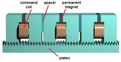
Fig. 3.
Its working principle is shown in Fig. 4.
 |
||
|
a)
|
b)
|
c)
|
|
Fig. 4.
|
||
If the command coil is not energised, Fig. 4a, the magnetic flux generated by the permanent magnet, Fpm, passes through the core branch parallel to the permanent magnet due to its smaller magnetic resistance. In this case there is no significant force produced. If the coil is energised, Fig. 4b, the command flux produced by it, Fc, directs the flux of the permanent magnet to pass through the air-gap and to produce significant forces. Due to the force the mover moves one step to minimise the air-gap magnetic energy, Fig. 4c.
The tooth pitch and the number of modules determine the motor's resolution. By advanced control strategies the resolution of positioning can be increased significantly.
The modular linear motor offers particularly strong benefits in those industrial applications where fast and accurate moves under heavy loads are required (flexible manufacturing systems, robotic systems, machine tools, conveying systems, linear accelerators, turntable drives, automated warehousing etc.).
Design of the modular linear motor
The modular linear motor's design presents some specific aspects because of its complex toothed structure and of the requirement to take into account the iron core saturation and permanent magnet operating point change.
The design algorithm and the afferent computer program elaborated by the researchers of this team mainly solve these problems, offering a useful tool for designers.
The proposed design procedure is based on several relationships obtained from a simplified analytical motor model and on some existing experience in this field. The analytical model basics of the motor is a simplified magnetic equivalent circuit (shown in Fig. 5) of the mover module and of the platen segment under it.
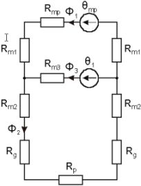
Fig. 5.
It consists two MMFs (q1 and qpm) of the command coil and of the permanent magnet. There are 9 reluctances in the circuit: Rpm of the permanent magnet, Rm1 and Rm2 of the pole, Rm3 of the core branch with the command coil, Rg of the variable air-gap and Rp of the platen segment under the mover module.
In the first stage of the design procedure the following required design inputs must be prescribed depending on the application in which the motor will be used:
The second stage is the main part of the design procedure. Here are established all the motor's dimensions. At the beginning the sizes of the toothed air-gap structure must be computed: the tooth pitch (function of the imposed positioning accuracy) and the air-gap length (that must be as small as mechanically possible). The selection of the best tooth geometry is very important, too.
The next step consists in choosing the active ferromagnetic materials used for the motor. Extremely important is the permanent magnet selection, the most expensive and sensitive assembly of the motor. The imposed temperature rise in the mover and the motor cost to performance ratio must be taken into account. Rare-earth magnets are needed to meet the high force per unit volume necessities of the motor. The magnet working point (Bpm, Hpm) on the straight demagnetisation characteristic throughout the second quadrant must ensure the desired flux density levels in the mover and platen cores.
The permanent magnet's dimensions can be determined by computing its minimal active surface and thickness:
 |
(1)
|
where Bp is the imposed flux density in the poles. The designing constant kp depends on the teeth pitch, respectively the slot width to air-gap length ratio (t/d and b/d). It can be easily determined from the three-dimensional diagram shown in Fig. 6.
Fig. 6.
In a similar way can be determined the length of the permanent magnet:
 |
(2)
|
where Br and Hc are the residual flux density, respectively the coercive force of the selected permanent magnet. The kx dimensioning constant can be chosen from a 3D diagram similar to that shown in Fig. 6.
Fig. 7.
The obtained dimensions of the magnet have to be rounded to actual data sheet values. After this a short iterative optimisation have to be made in order to find out the minimum volume of the magnet that is able to generate the required forces.
The control coil design have to be made as a function of its MMF (wI). It must be so great as to force all the permanent magnet's flux through the poles and the air-gaps. Also in this case a simple optimisation process can be applied. As numerous products of w and I can give the same MMF, it must be chosen that combination which will produce the less I2R loss in the command coil. This way both the electrical input and thermal dissipation of the command coil are minimised.
Next the sizes of the command coil must be determined. The coil length must ensure a distance equal to an integer multiple of the teeth pitch between the two poles. As the coil length and width imposes the yoke length, respectively the pole height, it is very important to choose in an optimal way the ratio of the two coil sizes. Beside this the coil width to length ratio must be prescribed in a manner to reduce as much as possible the leakage flux of the coil. As in this case there are also several possibilities to define the two main sizes of the command coil and there are three different requirements to fulfill, an optimisation process must be applied in order to define the best coil width to length ratio. Since the coil sizes impose the two of the main dimensions of the mover core, the most significant result of this simple optimisation can be the minimisation of the total core volume.
One of the most sensitive stages of the motor's design is the sizing of the core branch on which the command coil is placed. When the module is inactive, all the flux generated by the permanent magnet has to pass through this core element. While the command coil is energised the command flux produced has to concentrate the entire permanent magnet flux to pass through the poles and air-gaps. The analytical computation of this core branch is quite difficult due to its dependence of several items pending on other motor components. In this case an iterative field computation process was adopted in order to find out the best cross-section of this core branch (its length is imposed by the length of the command coil).
The rest of the sizes of the mover module and of the platen are computed just like in the case of the classical hybrid stepper motor, presented in detail in [1].
As it was stated out, the step length of the motor depends also on the number of modules coupled to form the mover (N). Due to this is very important to ensure the required distance between two mover modules. Beside this the spacers placed between the modules have to avoid direct magnetic coupling through the leakage fluxes of the two modules. In conclusion the following expression must be considered for the spacer length:
|
|
(3)
|
This was the last part of the design algorithm.
The main dimensions of the sample motor's module are given in Fig. 8.
Fig. 8.
The most significant characteristics of the sample motor are given in Table I.
Table I.
|
Number of modules |
3 |
|
Number of teeth per pole |
5 |
|
Tooth width |
0.84 mm |
|
Slot width |
1.16 mm |
|
Tooth pitch |
2 mm |
| Step size |
0.66 mm
|
|
Permanent magnet type |
VACOMAX 148 |
|
Residual flux density |
0.9 T |
|
Coercive force |
650 KA/m |
|
Turns number of the command coil |
400 |
|
Rated command current |
1 A |
|
Maximum tangential force |
150 N |
|
Motor width |
83 mm |
|
Air-gap |
0.1 mm |
The magnetic field analysis of the modular linear motor
The numeric field analysis of the three phase modular linear motor was performed by the FEM based MagNet 6.10 package (of Infolytica Inc.).
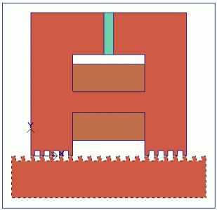
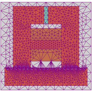
First only a single module with the platen part above it was analysed. Its solid model and the solution mesh generated by the program are shown in Figs. 9 and 10.
 |
 |
|
Fig. 9.
|
Fig. 10.
|
In Figs. 11 and 12 the obtained flux plots are presented for a passive, respectively active module. The module is in a relative position of x=0 mm. The command coil is fed by 0, respectively 1 A current.
|
Passive module
(unenergised command coil) |
Active module
(energised command coil) |
 |
 |
|
Fig. 11.
|
Fig. 12.
|
There is possible to represent the flux density distribution in the studied domain by using shaded plots. The magnitude of the flux density in each motor part can be determined by using the attached color maps. The shaded plots of flux density for the passive, respectively active module are given in Figs. 13 and 14.
|
Passive module
(unenergised command coil) |
Active module
(energised command coil) |
 |
 |
|
Fig. 13.
|
Fig. 14.
|
As it can be seen, the obtained results are perfectly in accordance with the theoretical expectations.
The numeric magnetic field analysis was also performed for the entire motor structure having 3 modules (Fig. 3). Of course the number of the generated elements (see Fig. 15 with the solution mesh of this problem) is about three times greater, therefore the computation time is also longer.
Fig. 15.
The FEM analysis of the three-phase modular linear motor was done for a one step displacement of the mover. The field analysis was performed for the following mover positions and command current values:
All the results obtained (the flux plots and the values of the total tangential and normal forces) are given in Table II.
Table II.
|
|
Data |
Flux plots |
Ft [N] |
Fn [N] |
|
a) |
x=0 mm Ic1=0 A Ic2=0 A Ic3=0 A |
|
0 |
105.48 |
|
b) |
x=0 mm Ic1=0 A Ic2=1 A Ic3=0 A |
|
135.3 |
417.59 |
|
c) |
x=0.25 mm Ic1=0 A Ic2=1 A Ic3=0 A |
|
111.13 |
807.6 |
|
d) |
x=0.5 mm Ic1=0 A Ic2=1 A Ic3=0 A |
|
81.3 |
810.6 |
|
e) |
x=0.66 mm Ic1=0 A Ic2=1 A Ic3=0 A |
|
3.23 |
1182.76 |
|
f) |
x=0.66 mm Ic1=0 A Ic2=0 A Ic3=0 A |
|
0 |
105.48 |
The variation of the flux lines distribution during one step displacement can be observed in an easy way. These results are also in good accordance with the theoretical expectations and with the analytical computations [11].
The control of the modular linear motor
There are several control possibilities for the three-phase modular linear motor from the simplest open-loop control schemes to the most sophisticated and powerful variable speed drive systems. In the last case the speed can be modified from zero to many meters per second. The motor's speed capability can be determined by design and depends on the supply frequency. The stopping, starting and reversing of the motor are all easy to implement. From the numerous possibilities available the right decision must be made as to trade off the overall cost of the control system, maintaining the required control capabilities.
Sensorless closed-loop operation with high demands regarding the control quality is one of the best solutions to be applied. It is based on the so-called back EMF detection of the un-energized command coils. The motor has three command coils, so there are always only one or two coils energised. Of course, in order to have continuous movement, the command coils needed for motion are always changing with the speed of the applied frequency, which means that the coils that are un-energized also change. The voltages induced in these coils provide an estimation of motor speed and position. The motor always starts from a well-defined initial position. In order to achieve maximum average tangential force (needed for the optimal efficiency) the command coils should always be energised at a precise moment, at the optimal commutation angle [2].
In this case the operating frequency will depend only on the capability of the motor to make a step under given conditions as load and input source limits. The speed controller commands the compact converter in function of the mover's position and speed. In such a way minimal current value is requested to obtain the necessary high tangential force. One limiting factor for the use of the back EMF detection is that the motor must have a minimal speed so that the "unused" coils to be able to trigger the detection circuit.
As it was previously pointed out, to achieve maximum average tangential force and to reduce as much as possible the tangential force ripple the control system has to assure the change of excitation of the three module's command coils at a specific displacement, the optimal commutation angel (ao), before reaching the intermediate equilibrium points. This value may be determined theoretically and depends on the number of modules coupled together to form the mover. For a three-phase modular linear motor the optimal commutation angle is ao=-17.46°. The two different commutation strategies are illustrated in Fig. 16 (the computations were made for another motor than the sample one presented above) [7].
|
Commutation at the intermediate equilibrium position
(a=0)
|
Commutation at the optimum commutation angle (a=ao) |
 |
 |
|
Fig. 16.
|
|
The data in Table III. highlights the benefits of the proposed commutation strategy. As it can be seen, for the proposed commutation strategy the mean value of the produced tangential force is increased with 6.67% and the force ripple is reduced with about 40%.
Table III.
|
Tangential force [N] |
Commutation angle |
|
|
(a=0) |
(a=ao) |
|
|
Minimum value |
0 |
29.75 |
|
Maximal value |
74.4 |
74.4 |
|
Mean value |
53.39 |
56.95 |
|
Range |
74.4 |
44.65 |
Table IV. presents the sequence of energising the command coils for a displacement to the left, respectively to the right. In the initial position of the mover considered the teeth of the module 1 are aligned with the teeth of the platen. In the table the correspondence at each sequence between the supplied and the monitored un-energised coils (in which the back EMF is detected) are also given. As it can be seen, each time a single command coil is supplied. For all the supplied command coils corresponds a monitored coil in both direction of displacement [6].
Table IV
|
Direction of displacement |
|||||
|
Left |
Right |
||||
|
Sequence number |
Energised coil |
Monitored coil |
Sequence number |
Energised coil |
Monitored coil |
|
I. |
3 |
1 |
I. |
2 |
1 |
|
II. |
2 |
2 |
II. |
3 |
2 |
|
III. |
1 |
3 |
III. |
1 |
3 |
The motor can be energised simply from a low cost readily available modern standard three-phase compact converter. This is connected to the microcontroller-based intelligent speed control unit. The speed controller may be linked to PLCs or other control units (hosts) for general system supervision. A special unit detects the back EMF generated in the un-energised command coils. The whole control system is presented in Fig. 17.
Fig. 17.
In a standard three-phase compact converter the dc power supply is derived from the ac mains by rectification and smoothing. The output current is regulated by switching on or off the power devices (such as MOSFETs or IGBTs), which connect output to the internal dc bus. By its high efficient current feedback control system it allows fully independent precise control over the motor command coil's currents, so it can deliver precisely the current pulses as is required for the motor. It is simple to operate and to install or remove.
The three-phase modular linear motor cannot be simply supplied from the standard three-phase converter. The three command coils must be connected in a delta connection, with diodes placed in series with each winding. Bi-directional command currents are not necessary since the generated tangential force is not function of the command current's polarity.
In this control system the standard converter and motor are perfectly harmonised with one another. The converter can assure high degree of efficiency because it can save and carry out several sophisticated positioning programs for different (standard and non-standard) motor types due to the full range of features included. In addition the standard converter has a whole series of supplementary internal functions (input protection, temperature and current sensing), which are special benefits for the entire control system.
Due to its great computation capabilities the intelligent speed/force controller is an integral part of the control system. It remotely supervises the converter by a serial communication link. The controller provides the built-in controller of the converter with the reference current signal, obtained from reference speed input and the direction of movement, and with the estimated displacement of the mover. This is computed from the detected EMFs via a specific algorithm.
The converter's controller generates the PWM command signals of the inverter and also picks up from a table the proper current pulses pattern, function of the movement direction and the mover's actual position. One of the inputs for this control stage is the measured current obtained from a sensor placed in the intermediate dc circuit of the power converter.
The proposed control strategy has to be implemented using the adequate assembler language shared on the compact converter's built-in controller and on the speed/force controller unit.
A mathematical model of an electric machine is based on a theoretical approach and can be used for easy performance prediction and control without prototyping. To be useful the model must be realistic and yet simple to understand, easy to manipulate and implement. The development of a practical model is not easy, because the above mentioned requirements are conflicting. Therefore a skillful mathematical model of a certain electrical machine can be very useful for prediction of its behaviour both in transient and steady state regime, and for testing several control schemes.
The best suited mathematical model for simulating the dynamic regime of a modular hybrid linear motor is a coupled circuit-field one. Its block structure is given in Fig. 18.
Fig. 18.
As it can be seen from the figure the model is composed of three interconnected submodels [1].
The first submodel consists of the circuit-type equation. The command currents are computed using the voltages of the command coils and taking into account the variation of the inductances due to the flux modifications in them.
The field submodel is based on the equivalent magnetic circuit of the motor. Obviously the field problem may be solved via a numerical method, using finite elements or finite differences methods, but these are very time consuming. Therefore the equivalent magnetic circuit method approach was applied.
The iron core nonlinear magnetic characteristics are characterized by computing the nonlinear permeances of the motor iron core portions taking into account the field-dependent single valued permeability . The dependence of this permeability is obtained by calculus at each iteration from the given magnetizing characteristic of the iron core material. The variation of the air-gap magnetic reluctances under the motor poles function of the mover position are considered, too.
The electromagnetic forces can be evaluated either from the gradient of the magnetic co-energy with respect to a virtual displacement or by Maxwell's stress tensor method. The former method is more reliable for this problem and it was adopted here.
The mechanical submodel considered here is a simplified one. In order to obtain this model two assumptions were made: the motor is considered as a homogeneous solid, the resulting tangential and normal forces being applied on its center, and the resulting forces are obtained as an algebraic sum of the pole forces. This simplified mechanical model does not take into considerations the torques that exist. These torques are produced by the normal forces that are not applied in the center of the mover but in each pole axis. By solving the above force equation the velocity and displacement of the motor are computed [1].
This coupled circuit-field model can not be solved analytically. The computational process consists of a simultaneous iterative calculation of the circuit type equations, of the field problem and of the equation of the movement [5].
In order to increase the accuracy of the simulations and to reduce the simulation times an enhanced model was applied for the dynamic simulations of the modular linear stepper motor in discussion.
The different parts of the model are implemented in different simulation platforms (SIMULINK, SIMPLORER and MagNet), each one of them being widely used in its field. Hence the main advantages of each platform were exploited, and the global efficiency of the entire simulation program is almost as high as possible. The block diagram of the coupled model is given in Fig. 19 [12].
Fig. 19.
One of the units is a finite element method (FEM) based magnetic field analysis module. Upon these computations, made in MagNet 6.0 off-line the simulations, the static characteristics of the motor are computed: the total tangential and normal forces of the motor for different command currents and mover positions. In order to determine these characteristics several computations were made for different control currents (in the range of 0÷2 A) and distinct relative displacements of the mover with a step of 0.1 mm were considered. The obtained static characteristics are given in Fig. 20.
|
Static characteristics |
|
 |
 |
|
Fig. 20.
|
|
The results are stored in look-up tables to be used in the main SIMULINK unit. The FEM analysis is far the most precise method for determining these characteristics. It is time consuming, but these computations must be done only once for a given motor. The use of the static characteristics of the forces instead of their in-line computation shortens considerably the simulation times.
The power converter feeding the command coils of the three-phase modular linear motor was modelled in SIMPLORER. This software package is frequently used for simulating comprehensive electric circuit components. SIMPLORER is very user-friendly, due to its graphic interfaces making even complex models easy to define [13].
The power converter unit is composed of three independently working one-phase inverters, built up using power transistors. The SIMPLORER model of the single phase H-bridge inverter is shown in Fig. 20.
Fig. 21.
The so-called SIM2SIM SIMPLORER-SIMULINK coupling's interface allows the exchange of each variable between a SIMPLORER and a SIMULINK model. The parameter exchanges are clearly arranged, so the different system quantities can be linked easily and quickly. During the simulation an automatic step width control in SIMPLORER and SIMULINK takes place. The parameters set in SIMPLORER are given in Fig. 22.
Fig. 22.
The coupling element in SIMULINK is an S-Function-type block. After a multi-step setting process the link between the two different simulation platform can be easily established.
The basic part of the coupled simulation program is implemented in MATLAB/SIMULINK. As it is well known, this environment is one of the best suited for the dynamic simulation of electrical machines.
The main window of the simulation program is given in Fig. 23.
Fig. 23.
As it can be seen, it is built up in a modular manner (using several sub-system type blocks). All the main components of the linear drive system can be clearly distinguished in the model. This way high transparency was assured for the users. Hence any changes in the program can be made quickly and easily. The program calls several MATLAB functions, e.g. for the setup (when the motor's main parameters are loaded from an M-file) or for the final plotting of the results. All the benefits of MATLAB (easy to write program lines, advanced graphical visualisations) and of SIMULINK (simple modular model building, easy to use graphical interface, etc.) are fully exploited.
The motor model subsystem is given in Fig. 24. This is also built up modularly: a subsystem is generating the three imposed command currents. In this subsystem are included the three S-Function type blocks obtained by the SIM2SIM linkage with SIMPLORER. These blocks are modelling the power converters feeding the command coils of the linear motor.
Fig. 24.
The models of the three modules of the motor were also grouped in a separate block (called Module 1, etc.) and are shown in Fig. 25.
Fig. 25.
Each block corresponding to a mover module has 3 inputs (the command current, the mover's displacement and the module's relative position within the mover armature) and two outputs (the tangential and the normal force). The forces of each module are added in order to obtain the total tangential and normal forces of the motor. In the subsystem called Mechanical system the speed and the displacement of the motor are computed. These are the output signals of the entire model of the motor.
The values of the forces for certain currents and displacements are interpolated from two look-up tables, containing the results of the magnetic field analysis performed by the FEM based MagNet program. As it can be seen, the drawings on the mask of the look-up table type blocks are just the static characteristics shown in Fig. 20.
The above-presented coupled model was used for simulating several dynamic regimes of the motor. Any of the motor characteristics could be obtained and plotted in order to make easy its study.
From the numerous dynamic regimes studied using this model of the three-phase modular hybrid linear stepper motor here only the results obtained for a short (10 mm long) displacement at controlled speed are given. A typical trapezoidal speed profile was imposed. The maximum speed of the motor was set at 0.25 m/s and the motor is running at this speed 0.02 s. The acceleration, respectively deceleration times were fixed to be 0.02 s. The sample three-phase motor's rated command current, respectively tangential force is 1 A and 135 N. Its step size is 0.66 mm.
The main results of the simulation are given in Fig. 26. The command currents, the total tangential and normal forces, the speed and the displacement are plotted versus time.
Fig. 26.
As it can be clearly seen in the figure the imposed speed profile was precisely followed. High tangential forces were needed for accelerating the mover. Due to the high force required for this stage of motion, the command currents also have significant values. After the mover was accelerated, low tangential forces obtained by feeding the motor with reduced command currents may maintain its imposed constant speed.
The use of the look-up tables reduced the computational times, because there was no need to calculate the total normal and tangential forces at each time step. Of course the filling out of these tables required several time-consuming field computations in MagNet, but these field analysis had to be made only once for a given motor. The simultaneous work of the two platforms (SIMULINK and SIMPLORER) and the exchange of variables at each time step inherently slow down the simulation. The lost time is compensated by the quality of the results. To emphasise this in Fig. 27 the current waveforms during a commutation are presented.
Fig. 27.
It can be seen very clear, that the current waveforms obtained by using the SIMPLORER converter model are much more appropriate of the real currents obtained by PWM techniques.
These results, as all others obtained for diverse dynamic regimes are in good accordance with the theoretical expectations and also with the results of analytical computations.
Surface motors assure two degrees of freedom movement in the plane. These are direct driven motors, the load can be put or fixed directly on the mover. Hence they have a lot of benefits, as the linear motors: simplicity, efficiency and positioning accuracy, due to the lack of rotary-to-linear conversion mechanisms, mechanically complex assemblies that require regular maintenance and develop inaccuracies over time.
In a typical application of the surface motors, the flexible manufacturing system, they carry the product subassemblies from one overhead manufacturing device to another and precisely position the subassembly so that the overhead devices can perform their required actions.
The structure of a typical surface motor is given in Fig. 28.
Fig. 28.
The modular surface motor, like any surface motor, consists of two main parts: the platen and the mover (forcer). The passive platen of steel has a two-dimensional array of square teeth obtained by precise chemical machining. Its surface is planarized using epoxy. It can have any sizes in order to ensure great travel area. The mover, the active part of the motor, is built up of high force modules (see Fig. 2), just like the modular linear motors presented above.
Basically the mover is composed of two modular linear motors, each ensuring the movement in one of the two transitional directions. For easy control purposes a three-phase motor type was selected. This requires minimally 6 modules (3 for each direction). Three of the modules are mounted at 90° to the other in a common housing. One set of coils drives the forcer in the x direction and the other in the y direction. The simplest mover structure having 6 modules is given in Fig. 29.
|
The 3D structure of the mover
|
The arrangement of the modules |
 |
 |
|
Fig. 29.
|
|
In order to reduce the skew of the mover due to undesired rotational moments a symmetrical structure must be selected. This has totally 36 modules arranged perfectly symmetrical in the mover unit (see Figure 30.). Every phase of the two motor parts (x1, x2 and x3, respectively y1, y2 and y3) is compound of six modules coupled in parallel power supply. The mover unit built up in this manner can develop high (several hundreds on N) force on both directions [9].
Fig. 30.
Compressed air flows through the mover, creating a high stiffness air bearing. Thus a uniform, narrow air-gap can be maintained between the platen and the mover in the presence of great attraction forces. Due to the air bearing there are no moving parts and no wear, resulting in greater long-term system accuracy and minimal maintenance.
The modular surface motor has several advantages as its linear counterpart: by using the specified mover modules one of the main disadvantages of the classical hybrid linear motors (the presence of braking forces at each position) was eliminated. It has the ability to perform simultaneous accurate orthogonal motion in the two directions and to move anywhere on the platen surface. The mover due to the already mentioned great attraction forces can be mounted face up or inverted. Because of the permanent magnets presence in the forcer, that preload the pneumatic bearing, the motor can be inverted allowing the payload to hang below the motor. This means that the forcer can ride on top or on the bottom of the platen surface.
Applying a sophisticated multi-level control system more than one movers can share simultaneously a common platen providing a compact multiaxis assembly with overlapping trajectories.
The modular surface motor, in a same manner as the other planar motors can be used in numerous industrial and laboratory applications. Its most typical application is of pick and place type. For example the mover transports the sub-assembly from the feeder to a manipulator or overhead processors, they do the assembly operations and the finished part is carried to a container. Such of systems are used for instance in electronic industry (for PCB throughhole and surface mount assembly, adhesive dispensing or probing for various types of testing requirements) or in pharmaceutical industry (for automated clinical lab sample handling or for multi-head pick and place workcells).
Control of the modular surface motor
Basically the modular surface motors are a sort of combination of two linear stepper motors. Hence these motors can be operated also in the open-loop mode. Nevertheless in this operating mode they can miss steps if large enough unanticipated external forces are acting. Controlled in this manner the motors have long settling times and low disturbance rejection. Also there is no possibility to provide controlled forces and high stiffness. They fall short of their potential capabilities due to possible loss of synchronism. All these limitations of open-loop operation restrict their usefulness in a wide range high precision and accuracy application.
In order to enhance their overall performance (such as operation at high speed with high accuracy) as well as in improving the disturbance rejection properties of the motor it must be controlled in closed-loop mode. However its sophisticated, complex two axis movement requires a relatively complicated control systems, the supplementary cost of the closed-loop control system do not influence significantly the overall control costs.
Each motor part assuring the movement in one of the two transitional directions has to be controlled apart. A general planar motion system supervisor controller generates the imposed planar motion profile to be strictly executed. A x & y trajectory generator serves the two displacement regulators with the imposed displacement signals (see Fig. 31).
Fig. 31.
The two sets of control coils of the motor can be energised simply from two (one for each direction movement) low cost readily available modern standard three-phase compact converters. These are connected to the two microcontroller-based intelligent speed control units. In order to perform the so-called back-EMF detection sensorless operation the control system also has two special circuits to detect the back EMF generated in the un-energised command coils.
In order to achieve maximum average tangential force the command coils should always be energised at a precise moment, at the precisely computed optimal commutation angle, before an intermediate equilibrium position to be reached, just like their linear counterparts.
Dynamic simulation of the modular surface motor
The proposed surface motor's dynamic behaviour was studied using a high performance coupled simulation program. The program is an extension of the simulation program of the modular linear stepper motor [8]. Its main window is given in Fig. 32.
Fig. 32.
The subsytems used for this model are the same as those used for simulating the modular linear stepper motor.
The simulated task was a typical pick and place type application. The mover starts without load from its initial position, A, and moves into position B. Here the load is put on the mover and it is displaced in C. Here the load is taken down and the motor returns to its initial position (see Fig. 33). Three trapezoidal speed profiles must be generated for each sequence of the movement.
Fig. 33.
The main results of the simulation for the part of the motor that ensures the displacement in x direction is shown in Fig. 34. The command currents, the total tangential and normal forces, the speed and the displacement are plotted versus time.
Fig. 34.
As it can be clearly seen in the figure, all the three imposed speed profiles were closely followed up. High tangential forces were needed for accelerating the mover. Due to the high force required the command currents for this stage have also significant values. After the mover was accelerated its imposed constant speed may be maintained by low tangential force. To emphasise the accuracy of the drive system its speed error for axis x) is given in Fig. 35.
Fig. 35.
Also upon this figure it can be concluded that the above presented sensorless closed-loop control system guarantees the highest demands regarding the quality of the planar motion.
![]()
Main papers published in this field (arranged by time):
Viorel I.A. - Szabó L.: Hybrid Linear Stepper Motors, Mediamira Publisher, Cluj-Napoca (Romania), 1998. ISBN 973-9358-12-8
Viorel I.A. - Szabó L.: Permanent-magnet variable-reluctance linear motor control, Electromotion, vol. 1., nr. 1. (1994), pp. 31-38.
Szabó L. - Viorel I.A. - Chişu I. - Kovács Z.: A Novel Double Salient Permanent Magnet Linear Motor, Proceedings of the International Conference on Power Electronics, Drives and Motion (PCIM), Nürnberg, 1999, vol. Intelligent Motion, pp. 285-290.
Viorel I.A. - Szabó L.: A Modular Hybrid Linear Stepper Motor, Proceedings of the 5th Conference on Engineering of Modern Electric Systems, EMES '99, Băile Felix (Romania), published in the Oradea University Annals, Electrotechnics Section (C), pp. 187-192.
Szabó L. - Viorel I.A. - Józsa J.: Dynamic Simulation of a Novel Hybrid Linear Stepper Motor by Means of Matlab/Simulink, Proceedings of the International Conference on Renewable Sources and Environmental Electro-Technologies RSEE '2000, Băile Felix (Romania), published in the Oradea University Annals, Electrotechnics Section, 2000, pp. 49-54.
Szabó L. - Viorel I.A.: An Integrated CAD Environment for Designing and Simulating Double Salient Permanent Magnet Linear Motors, Proceedings of the International Conference on Power Electronics, Drives and Motion (PCIM), Nürnberg, 2001, vol. Intelligent Motion, pp. 417-422.
Viorel I.A. - Szabó L.: On a Three-Phase Modular Double Salient Linear Motor's Optimal Control, Proceedings of the 9th European Conference on Power Electronics and Applications (EPE), Graz (Austria), 2001, on CD: PP00237.pdf.
Szabó L. - Dobai J.B.: Combined FEM and SIMULINK Model of a Modular Surface Motor, Proceedings of the IEEE-TTTC International Conference on Automation, Quality and Testing, Robotics A&QT-R 2002 (THETA 13), Cluj, tome I., pp. 277-282, on CD: 1_2_29_Szabo Lorand.pdf.
Szabó L. - Viorel I.A.: On a High Force Modular Surface Motor. Abstract in Proceedings of the 10th International Power Electronics and Motion Control Conference (PEMC '2002), Cavtat & Dubrovnik (Croatia), 2002, pp. 384. Paper on CD: T8-052.pdf.
Szabó L. - Viorel I.A. - Szépi I.: FEM Analysis of a Three-Phase Modular Doubly Salient Linear Motor, Proceedings of the Workshop on Variable Reluctance Electrical Machines, Cluj, 2002, pp. 48-51.
Szabó L.: Field Analysis of a Three Phase Modular Double Salient Linear Motor by Means of FEM, Oradea University Annals, Electrotechnical Section, 2002, pp. 72-77.
Szabó L. - Viorel I.A. - Dobai J.B.: Multi-Level Modelling of a Modular Double Salient Linear Motor, Proceedings of the 4th International Symposium on Mathematical Modelling (MATHMOD '2003), Viena (Austria), pp. 739-745, on CD: 115-Text-Lorand-Szabo.pdf.
For comments and suggestions feel free to contact the authors.
Last modified on:
January 29, 2008